
Introduction
Most manufacturers have a schedule. The problem is that the schedule lies.
Work orders get released based on due dates, but nobody checks whether the CNC machining center is already booked solid for the next two shifts. The result is predictable: jobs pile up at the same bottleneck machine, overtime spikes every Friday, and the planning team spends its week rescheduling yesterday's problems instead of planning tomorrow's production.
This isn't a discipline problem — it's a method problem. Infinite capacity scheduling, the default logic in most ERP and MRP systems, assumes resources are always available. It answers "what do we need to make?" without asking "do we actually have the capacity to make it?"
Finite capacity scheduling (FCS) answers the second question. It assigns every work order to a specific machine, in a specific time window, based on what that machine can actually handle: shifts, maintenance windows, changeovers, and operator availability all accounted for.
This guide covers what FCS is, how it differs from infinite scheduling, how the core scheduling logic works, its operational benefits, and how to implement it effectively on a real shop floor.
Key Takeaways
- FCS assigns jobs only to slots where capacity actually exists — no double-booking, no overloads hidden on paper.
- Infinite capacity scheduling (standard in most ERP/MRP systems) ignores real constraints, so overloads stay invisible until they hit the shop floor.
- Core FCS approaches include forward scheduling, backward scheduling, constraint-based/DBR, APS, and JIT.
- Without live machine data, a static FCS schedule loses accuracy fast; real-time connectivity is what keeps it reliable.
- Best practices: nail your baseline capacity data, prioritize bottleneck resources when scheduling, and tie the schedule to live machine status.
What Is Finite Capacity Scheduling?
Finite capacity scheduling is a production planning method that assigns work orders to machines and work centers based on their actual available capacity during a given time window. It accounts for shift patterns, planned maintenance, tool availability, changeover durations, and operator hours — not a theoretical assumption that resources run at 100% utilization indefinitely.
"Finite" simply means bounded by reality. That boundary is what makes it actionable — and understanding where it sits relative to broader capacity planning is where most shops start.
Scheduling vs. Capacity Planning
The terms finite scheduling and finite capacity planning are often used interchangeably in manufacturing operations, but there's a useful distinction:
- Finite capacity planning — the broader strategic exercise of managing production within defined resource limits
- Finite capacity scheduling — the operational sequencing and timing of individual jobs against those limits
On the shop floor, the two function as a single integrated loop: planning sets the constraints, scheduling works within them.
The Core Output
FCS answers one question: Given what we actually have available right now, when can each order realistically start and finish?
That's entirely different from an ERP plan that tells you what needs to happen without verifying whether the capacity exists to execute it. ERP tells you what the plan requires. FCS tells you whether your machines, operators, and tooling can actually deliver it — and adjusts the schedule when they can't.
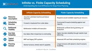
Finite vs. Infinite Capacity Scheduling: Key Differences
Most ERP and MRP systems use infinite capacity scheduling by default. The logic is straightforward: pick a due date, backward-schedule through each operation, and release the work order. Whether the machine is already fully loaded doesn't factor in.
This isn't a flaw in ERP design — infinite capacity logic is the right tool for material requirements planning. It answers "what materials do I need to order and when?" accurately. The problem starts when manufacturers rely on that same logic to run their shop floor.
The Operational Gap
When the CNC machining center is already at 95% utilization and three more orders land on it simultaneously, infinite scheduling doesn't alert anyone. The overload only becomes visible when the shop floor can no longer execute — at which point the planning team scrambles, overtime gets authorized, and customer delivery dates slip.
According to the Manufacturing Leadership Council, 70% of manufacturers still enter data manually — meaning capacity information is often stale before planners even see it, compounding the gap between the planned schedule and shop floor reality.
Direct Comparison
| Dimension | Infinite Capacity Scheduling | Finite Capacity Scheduling |
|---|---|---|
| Resource assumption | Unlimited availability | Actual available capacity |
| Scheduling direction | Backward from due date | Forward into available slots |
| Bottleneck visibility | Hidden until execution | Visible before release |
| Due date reliability | Aspirational | Achievable |
| Typical system | ERP / MRP | APS / dedicated FCS module |
| Planning horizon | Medium to long term | Short to medium term |
Where FCS Fits in the Stack
ERP/MRP operates at the business planning level — managing orders, materials, and financials. FCS operates at the execution level, sequencing individual operations against real machine capacity. The two are complementary, not competing.
Problems arise when manufacturers try to make ERP do both jobs. FCS doesn't replace ERP: it closes the gap between what ERP plans and what the shop floor can actually deliver.
That distinction matters for throughput, too. FCS doesn't mean turning away orders or reducing output. It means scheduling orders into slots where capacity genuinely exists. That may extend a delivery date, but it produces a commitment the shop floor can honor — far more valuable than a date that looks good on paper and fails in production.
How Finite Capacity Scheduling Works: Types and Scheduling Logic
FCS algorithms place each operation into the first available capacity slot on the assigned resource, then link dependent operations in sequence. A time fence (the period within which finite constraints are enforced) defines how far forward the system actively manages capacity. Setting that window appropriately for your production cycle matters; too short and you're always reacting, too long and the schedule becomes too rigid to accommodate real demand changes.
The Five Primary FCS Approaches
| Approach | How It Works | Best For |
|---|---|---|
| Forward Scheduling | Plans from today forward; finds earliest completion | Flexible start dates, make-to-stock |
| Backward Scheduling | Plans from due date backward; minimizes idle time | Fixed deadlines, engineer-to-order |
| Constraint-Based / DBR | Bottleneck (drum) paces all other operations; buffers protect the constraint | Clear single bottleneck environments |
| Advanced Planning & Scheduling (APS) | Multi-variable algorithms optimize across many constraints simultaneously | Complex multi-constraint or multi-site operations |
| Just-in-Time (JIT) | Times production to arrive exactly when needed | Repetitive manufacturing, lean environments |
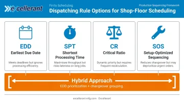
Dispatching Rules at the Bottleneck
Once FCS identifies the bottleneck, it sequences jobs using dispatching rules. Common approaches:
- Earliest Due Date (EDD) — sequences by due date; protects on-time delivery but can strand short jobs behind long ones
- Shortest Processing Time (SPT) — clears short jobs first; maximizes throughput count but risks late delivery on complex orders
- Critical Ratio (CR) — compares time remaining to work remaining; dynamically reprioritizes as conditions shift
- Setup-optimized sequencing — groups jobs to minimize changeover time; reduces OEE losses but can conflict with due dates
Most shops end up with a hybrid: jobs grouped for changeover efficiency within an EDD-prioritized window. That balance captures most of the changeover savings without sacrificing delivery performance.
Why Static Schedules Fail — and What to Do About It
A schedule built Monday morning starts degrading by Monday afternoon. Machine breakdowns, extended changeovers, material delays, and urgent order insertions all force revision of a pre-established plan. Dynamic scheduling research confirms that manufacturing scheduling is inherently reactive because new shop-floor information continuously invalidates prior assumptions.
The solution is connecting FCS to live machine data. When the scheduling model receives real-time inputs, it updates slot availability automatically — no planner needed to manually reconcile the gap. Those inputs include:
- Real-time machine run states and cycle times
- Downtime events and fault codes
- Actual OEE performance vs. planned capacity
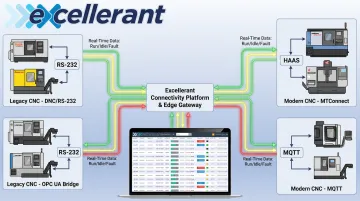
Excellerant's Finite Dynamic Scheduler closes this loop directly: it pulls live machine status and OEE feedback from its monitoring platform so the schedule reschedules against actual shop-floor conditions rather than static capacity assumptions. Legacy CNCs (connected via RS-232/serial adaptors) and modern machines (via ethernet or WiFi) feed into the same platform, so the scheduler reflects the full shop floor regardless of machine age.
FCS in Action: A Simple Example
Consider a two-step job: CNC machining followed by inspection and assembly.
With infinite scheduling: A new order for 50 parts arrives. The system backward-schedules from the due date and releases the work order — without checking that the CNC center is already committed for the next two shifts. The machine queue becomes triple-booked. Two of the three jobs will be late.
With finite scheduling: The FCS system checks actual available hours across the next three shifts, finds the first open capacity window (say, Thursday morning), slots the job there, and returns a confirmed start and finish time. The other two jobs already in queue are protected. The customer gets a date the shop can keep.
Finite scheduling's value is straightforward: the schedule reflects reality before it reaches the floor.
Benefits of Finite Capacity Scheduling
Operational Benefits
The most immediate gain is reliable delivery commitments. When due dates are calculated against actual capacity, promises to customers reflect what the shop floor can genuinely execute — not what an ERP assumed at order entry.
Beyond delivery accuracy:
- Prevents resource overloads — jobs are never double-booked onto a machine already at capacity
- Cuts firefighting time — planners focus on planning, not re-sequencing a queue that collapsed overnight
- Reduces unplanned overtime — overloads surface before they become weekend emergencies
WIP and Efficiency Gains
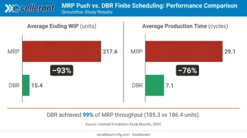
A 2019 DAAAM simulation study comparing MRP push, Kanban pull, and Drum-Buffer-Rope (DBR) scheduling illustrated the WIP impact clearly. DBR achieved 99% of MRP's throughput (185.3 vs. 186.4 finished products) while cutting average ending WIP from 217.6 units to just 15.4 and average production time from 29.1 cycles to 7.1 cycles.
FCS only releases jobs into the queue when the downstream resource is ready — so work doesn't pile up in front of a bottleneck waiting for a machine that won't be free for two days.
Setup-optimized sequencing at the bottleneck also reduces changeover losses — a meaningful OEE improvement in high-mix environments where changeovers consume a significant share of available machine time.
Strategic Value in Regulated Industries
For aerospace, defense, and medical device manufacturers, the stakes around delivery reliability are high. Raytheon's Supplier Rating System sets "Performing" OTD at ≥95% and "Underperforming" below 90%, with ratings refreshed twice monthly on a rolling 12-month window. Lockheed Martin explicitly uses supplier OTD data to inform future sourcing decisions.
What that means in practice:
- Suppliers missing the 90% OTD floor risk losing future work — not just a scorecard mark
- Sales teams can quote lead times with confidence when schedules reflect actual capacity
- Manufacturers can defend scorecard ratings with a process aligned to shop floor reality
How to Implement Finite Capacity Scheduling: Best Practices
Step 1 — Establish Accurate Baseline Capacity Data
No scheduling algorithm produces reliable output from bad input. Before implementation, document:
- Shift patterns and available hours per work center
- Planned maintenance windows and average duration
- Realistic run rates per machine and job type (not ERP standard times, which diverge from actual cycle times)
- Average changeover durations by job family
Excellerant's OEE and downtime tracking module captures actual cycle times, run/idle states by shift, and downtime reasons directly from the machine — giving planners measured data rather than estimates entered years ago when the routing was first built.
Step 2 — Identify and Schedule Bottleneck Resources First
Apply the Theory of Constraints principle: find the one or two resources that constrain overall throughput and schedule those first. Every other resource should be subordinated to the bottleneck schedule.
Skipping this step undermines everything downstream. Optimizing non-bottleneck resources without protecting the bottleneck yields no measurable improvement in system output — it only lengthens the queue in front of the constraint.
Step 3 — Match the Scheduling Approach to Your Production Profile
- High-mix, low-volume job shops → constraint-based scheduling with setup-optimized sequencing
- Repetitive or flow-line manufacturers → backward scheduling with JIT principles
- Multi-site or multi-constraint environments → APS with multi-variable optimization
Don't default to whatever the ERP provides. The scheduling method should reflect actual production structure, not system defaults.
Step 4 — Connect the Schedule to Real-Time Machine Data
A schedule built on stale capacity data fails on the floor. Integrate live machine status — run/idle/fault states, actual cycle times, downtime reasons — so the schedule updates when conditions change rather than requiring a planner to manually re-sequence after every disruption.
Excellerant's machine connectivity platform links legacy CNCs and modern machines into a unified real-time data feed. Legacy equipment connects via RS-232, serial, and PLC adaptors; modern CNCs use MTConnect, OPC-UA, Fanuc FOCAS, HAAS MNET, or Mazak Mazatrol. When a machine goes down or a job runs long, the schedule adjusts automatically — planners respond to exceptions rather than rebuilding the plan from scratch.
Step 5 — Build In Buffers and Measure Continuously
Add buffer time at bottleneck resources to absorb variability. Then track performance against these KPIs:
- Schedule attainment rate — percentage of jobs completed in the scheduled window
- On-time delivery — actual vs. committed ship dates
- Average lead time — whether FCS is compressing or extending cycle times
Treat FCS as an iterative system. Each deviation is data — use it to refine standard times, identify chronic bottlenecks, and improve future scheduling accuracy.
Common Challenges in Finite Capacity Scheduling
Data Accuracy
FCS is only as reliable as the capacity data feeding it. Inaccurate standard times and missing downtime records cause the schedule to diverge from reality almost immediately. The fix is automating data collection directly from machines rather than relying on manual entry — which the Manufacturing Leadership Council found still occurs at 70% of manufacturers.
Dynamic Demand and Disruptions
Urgent orders, customer reschedules, and unexpected breakdowns constantly invalidate even a well-built schedule. Three tactics help:
- Shorten the scheduling horizon (reschedule frequently in short cycles)
- Use Critical Ratio dispatching to dynamically reprioritize as conditions shift
- Establish a clear protocol for inserting urgent orders without cascading disruption through the entire queue
Stakeholder Resistance
Data and operational challenges aside, the people side of FCS is often the hardest to solve. Moving from infinite to finite scheduling changes how orders are promised, how the shop floor communicates with planning, and how performance is measured.
Start with a pilot on the highest-impact bottleneck resource. Demonstrated gains in on-time delivery and reduced overtime build organizational confidence before expanding the system.
Frequently Asked Questions
What does finite capacity scheduling mean?
Finite capacity scheduling assigns work orders to machines and work centers based on their actual available capacity (accounting for shifts, downtime, tooling, and changeovers) rather than assuming unlimited throughput. Every scheduled commitment reflects what the shop floor can realistically execute, not what looks achievable on paper.
What is an example of finite capacity scheduling?
A new order for 50 machined parts arrives. The FCS system checks the CNC machining center's actual available hours across the next three shifts, finds the first open capacity window, and slots the job there, returning a confirmed start and finish date based on what's actually open in the queue.
What is the difference between finite and infinite capacity scheduling?
Infinite capacity scheduling plans against a due date without checking whether resources are already fully loaded, which is the default logic in most ERP/MRP systems. Finite capacity scheduling places each job only into slots where capacity actually exists, making overloads and delivery risk visible before they reach the shop floor.
When should a manufacturer switch from infinite to finite capacity scheduling?
Key warning signs: chronic missed due dates despite a schedule that looks achievable on paper, repeated overtime on the same machines, constant re-planning firefighting, and growing WIP inventory.
Does finite capacity scheduling replace ERP or MRP?
No. ERP handles material requirements and order release: what to make and when to procure materials. FCS handles shop floor execution sequencing — which machine, which order. Running both together means your planned schedule matches what the shop can actually deliver.